Decision-Focused Evaluation of Worst-Case Distribution Shift
Predictions often decide who gets a scarce resource. If you search for the data change that hurts accuracy most, have you found the change that hurts those decisions most?
key idea what the paper found what is lost, or a limit
chapter 1
The question in one picture
A model is trained on one set of data and then used on another. The paper calls the difference a distribution shift. §1 A common way to test a model is to search for the worst-case distribution shift of a set size: the change that makes its loss largest. §2
Most such searches use a loss that counts errors person by person. §1 But predictions are often used for resource allocation: they decide who gets a scarce resource. §1 The paper's own example is an emergency room with a limited treatment.
The paper's emergency-room example §1
Two kinds of patients arrive at an emergency room with a limited treatment. §1
Errors about type 1 rarely matter, because they almost never need the treatment. §1
A search for the worst shift in accuracy fills the room with type 1 patients. §1
But a room full of type 2 patients is where the treatment decision goes wrong. §1
A search that maximizes errors fills the room with type 1 patients. Almost none of them need the treatment, so even poor predictions lead to good decisions. §1 The hard case for the decision is a room full of type 2 patients. The model is more accurate for them. §1
So a model may be more robust than expected if errors do not flip the decision, and less robust if small errors do. §1
The answer, in short
- The paper builds a search for the worst case of the decision itself. §3
- On US census tasks, the worst case found for one loss was never noticeably worse on another loss than that loss's own worst case. §4.3
- A search on the error rate can miss most of the harm to decisions. On one task it found only 0.14 of the worst loss for the decision. Figure 1
In the emergency room example, why are errors on type 1 patients cheap?
Type 1 patients almost never need the treatment. So the right decision is nearly always "no", whatever the model predicts. §1
Why is type 2 harder for the decision even though the model is more accurate there?
Their need for treatment varies a lot. So the decision depends on fine distinctions, and small errors can change who is treated. §1
chapter 2
What you need first
Predict, then decide
In predict-then-optimize, a model first predicts numbers. Those numbers then go into a decision problem that picks the best action. App.A Here the action is who gets the resource. §2
Decisions are made for a whole group at once, such as all patients who arrive on one day. The paper calls such a group an optimization instance. §1 The decision for one person depends on who else is in the group. §1
Measuring a bad decision
The decision loss compares two decisions for the same group. One uses the true outcomes, and one uses the predictions. It is how much worse the second one is. §2 When "how much worse" means the difference of the two values, the decision loss is the regret. The paper also allows a ratio instead. §2
The simplest decision problem is top-k. Each group has k units of the resource. The k people with the highest predictions get them. The goal is to reach as many people who need it as possible. §4.1 The knapsack version adds a cost for each person, and the total cost has a cap. §4.1
Searching for the worst case
The distributionally robust optimization literature looks for the worst data mix within a set size, with loss counted one person at a time. §1 §2 The set is centered on the empirical distribution: each person counts equally, as observed. §3 A divergence measures how far a new weighting moves from it. Capping it caps the size of the shift. §3
What two decisions does the decision loss compare?
The decision made with the true outcomes, and the decision made from the predictions. §2
What does capping the divergence prevent?
Without a cap, the worst case could be any data at all. The cap keeps the shift to a size the user picks. §3
chapter 3
What the paper does
A shift at two levels
Standard methods treat people as independent. In an emergency room they are not. Seeing one patient with a respiratory illness makes more such patients that day more likely. §1 So the paper uses a hierarchical model: first pick a group, then pick people within it. §1 §3
The hierarchical model: two places a shift can act §3
Top level: a shift may make some optimization instances more common than in the data. §3
Lower level: inside each optimization instance, a shift may change the weight on each person. §3
Each optimization instance gets its own decision, made from the predictions for its people. §2
The search looks for the weights, within both limits, that make the decision go worst on average. §3
A shift can act at both levels. It can make some groups more common. It can also change the weight on each person within a group. §3 Each level has its own limit on the divergence, set by the user. §3 The search looks for the weights at both levels that make the average decision loss largest. §2 §3
This search is hard. One person's effect on the loss depends on who else is in the group. §2 The paper shows the problem has a special shape, DR-submodular, that simple step-by-step methods can handle. §3 It solves it with a version of the Frank-Wolfe algorithm, a step-by-step search. §3
How the search is solved
The DR-submodular result needs a feasible set that contains the zero vector. So the paper searches over offsets from the empirical distribution, where an offset of 0 means no shift. §3 It also subtracts 1 from the loss, so the loss it works with is never positive, and adds the 1 back at the end. The proofs use this form. §3 The paper proves the objective is DR-submodular in the offsets within each group (Theorem 3.3), with proofs in Appendix B. §3 App.B
Each step of the Frank-Wolfe algorithm calls a subroutine the paper names gradmax. It finds the allowed weighting that points most in the direction the loss rises. §3 The search samples many decision problems per step and uses momentum from earlier steps. §3 App.C
In the experiments, each group decision is made for 40 people. The appendix sets the two limits to 40 and 6.25. It calls them ρ1 and ρ2, so it does not say which is the group limit and which is the person limit. Each search runs 15 steps, with 35,000 sampled problems per step. App.D
The test bed
The data are US census surveys from the folktables package. §4 There are three tasks: predict employment, predict income, and predict whether income is above $50,000. §4 Help goes to people likely to be unemployed or to have low income. Each US state is one optimization instance. §4
The search runs for many models, states and losses: 75,000 worst cases per task. §4 Each worst case is then scored on every other loss. §4
The models
For each state, the paper trains two models per task. One uses an ordinary loss, cross entropy loss or mean squared error. The other uses SPO, which trains the model for the knapsack decision. §4 App.D That gives 300 models. App.D Employment uses logistic regression. Income uses a neural network with two hidden layers. App.D
Two kinds of loss
The paper calls a loss that adds up errors person by person a decision-blind metric. §4.3 It uses 1-accuracy and cross entropy loss (CE). For income it uses mean squared error (MSE). §4.1 A decision-based metric instead looks at the decision made from all the predictions together. §4.3 These are top-k, knapsack, and two more. The fairness-based loss measures how unequally the top-k decision serves racial groups. The utility-based loss scores how well a budget of money reaches people with low income. §4.1
Why does the shift act at two levels?
Whole groups can differ, such as patients on different days. People can also differ within a group. §3
What is the difference between a decision-blind metric and a decision-based metric?
A decision-blind metric adds up errors one person at a time. A decision-based metric scores the decision made from all the predictions together. §4.3
chapter 4
What they found
A worst case for one loss is less harmful on another
The paper scores each worst case on every loss. It divides each score by the worst value found for that loss. A 1.0 means as bad as the worst case found for that loss. Figure 1
Income classification: a worst case found for the error rate is scored on top-k. What share of the worst top-k loss do you think it reaches?
The part below opens after your guess.
Figure 1 from the paper: each worst case, scored on every metric Figure 1 open full size
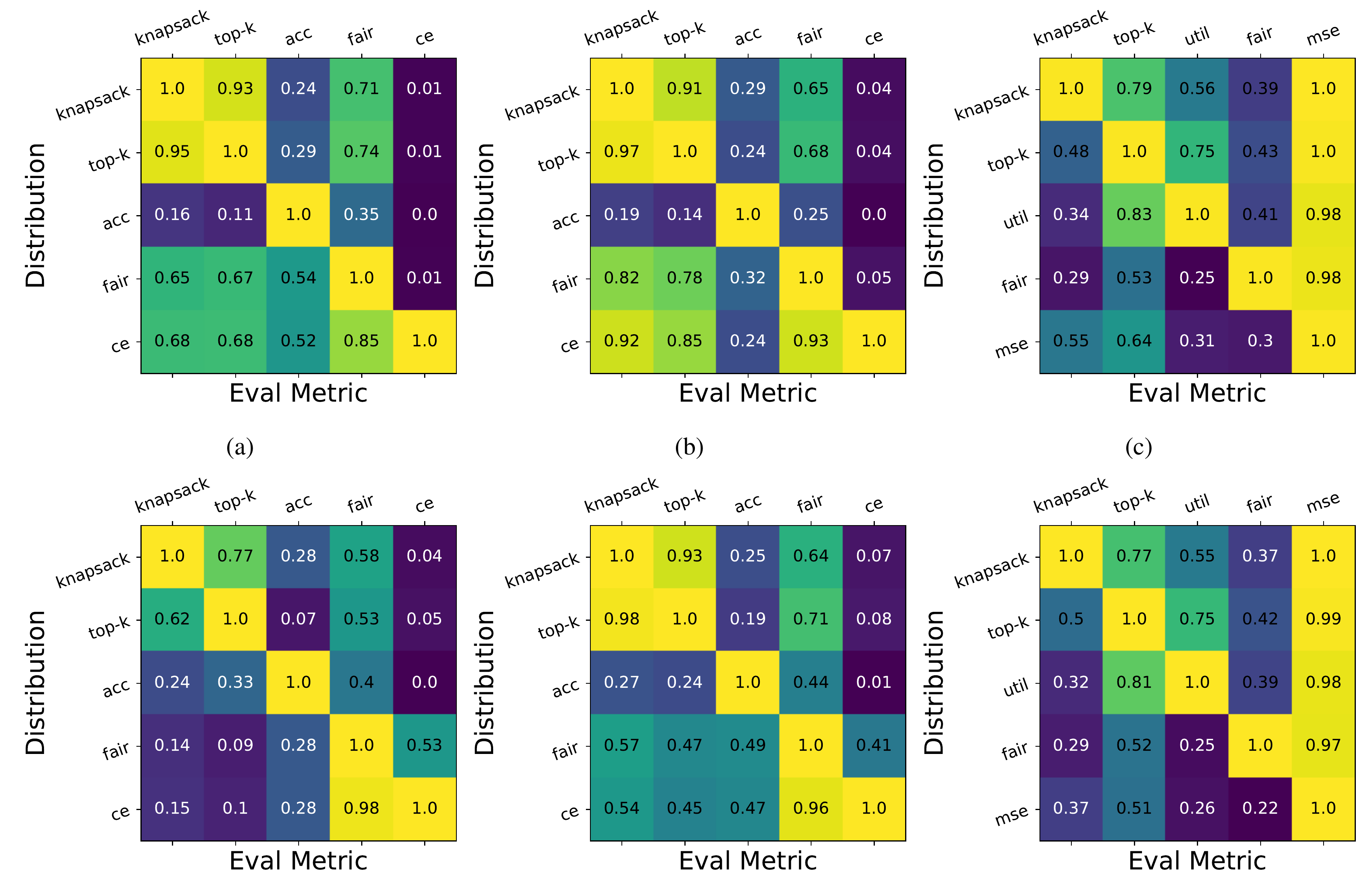
Panel a. Each row is the metric a worst case was found for. Each column is the metric it is scored on. Each column is divided by its diagonal cell, so the diagonal is all 1.0.
Panel b, income classification: the top-k column. Each cell is a worst case's top-k loss as a share of the worst top-k loss.
The worst case for the error rate, acc, reaches only 0.14 of the worst top-k loss.
Bottom row: models trained with SPO. The strong diagonal holds there too.
No cell is noticeably above the diagonal's 1.0 in its column. In the MSE column, many cells tie it at about 1.0. In the paper's words, no worst case "achieved a metric that was (noticeably) higher" than the one found for that metric. §4.3
Why a worst case for one loss can be mild for another §4.3
A made-up example: two groups of six people. Group A has two people who need the resource, group B one. The two highest predictions in each group get it. §4.1
The error rate counts every person on the wrong side of 0.5. Group A has 3 such errors, group B only 1. §4.1
With k = 2, group A's top two both need the resource, so its decision loss is 0. Group B's top two do not, and the one person who does, at 0.45, is missed. §2
The paper finds the same pattern at scale: a worst case built for 1-accuracy is mild for top-k. Figure 1
The size of the gap varies. For income classification, the worst case for CE reached 0.85 of the worst top-k loss. The one for 1-accuracy reached 0.14. Figure 1 App.E Worst cases for related decisions transfer well. The worst case for knapsack reached 0.97 on top-k. Figure 1
Income classification: which of these worst cases reached the most of the worst top-k loss?
The part below opens after your guess.
The paper concludes that decision-blind metrics risk underestimating the true worst case for decisions. §4.3 Changing the decision even slightly, such as giving each person a cost, can expose a model to shifts no one checked. §4.3
Two details in Figure 1
In the income regression panels, nearly every worst case scores about 1.0 on MSE. So for that loss, many searches found about the same worst value. Figure 1
The bottom row uses models trained with SPO. Its diagonal is also strong. Figure 1 The table in Appendix E gives each cell with its spread, for example 0.14 ± 0.007. App.E
Different worst cases pick different people
The paper then looks inside one state and one model. It plots each person's prediction against their weight in the worst case. §4.3
Figure 2 from the paper: who each worst case upweights Figure 2 open full size
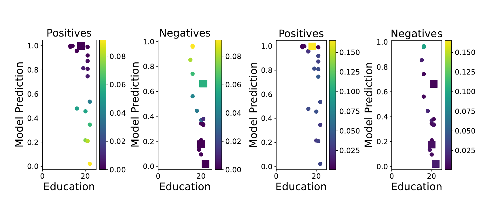
Panel a, the worst case for CE: high weight on an unemployed person predicted near 0 and an employed person predicted near 1 (positives = unemployed). The further wrong, the more weight.
Panel b, the worst case for the fairness-based loss: a non-white unemployed person with a high prediction gets high weight (square = non-white).
A white employed person with a high prediction also gets high weight (circle = white).
This is the employment task. A positive person is unemployed, and the prediction is the chance of being unemployed. A high prediction puts a person in the top k, so they get the help. §4.1 §4.3 For CE, weight grows with how wrong a prediction is: an unemployed person predicted near 0, or an employed person predicted near 1. §4.3 For the fairness-based loss, two kinds of people get high weight. One is a non-white unemployed person with a high prediction. The other is a white employed person with a high prediction. §4.3
These two make the decision serve non-white people correctly and white people incorrectly. That gap between groups is exactly what the fairness-based loss measures. §4.3 So the two worst cases put weight on different people. §4.3
Figure 3: the income regression task
Figure 3 from the paper: income regression Figure 3 open full size
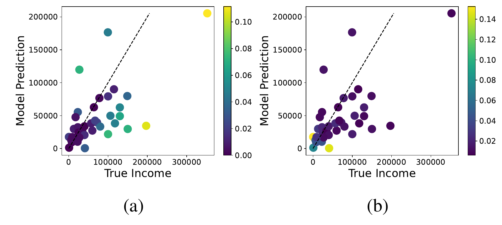
Panel a, the worst case for MSE: weight grows with the distance from the dotted line, where prediction equals true income.
Panel b, the worst case for the utility-based loss: the highest weights (yellow) go to two people with predicted income near zero. One of them earns more than predicted.
For MSE, weight grows with the gap between prediction and true income. §4.3 For the utility-based loss, only some large errors matter. Weight goes to people with a low predicted income but a higher true income. They take money that would help others more. §4.3 People with high true and high predicted income are not upweighted, even with large errors. They would not get money anyway. §4.3
Is the search close to the true worst case? Figure 4
With 8 people per group, an exact solver, Pyomo/IPOPT, can find the worst case. The paper compares its search to that answer. §4.3 App.D
Figure 4 from the paper: the method against an exact solver Figure 4 open full size
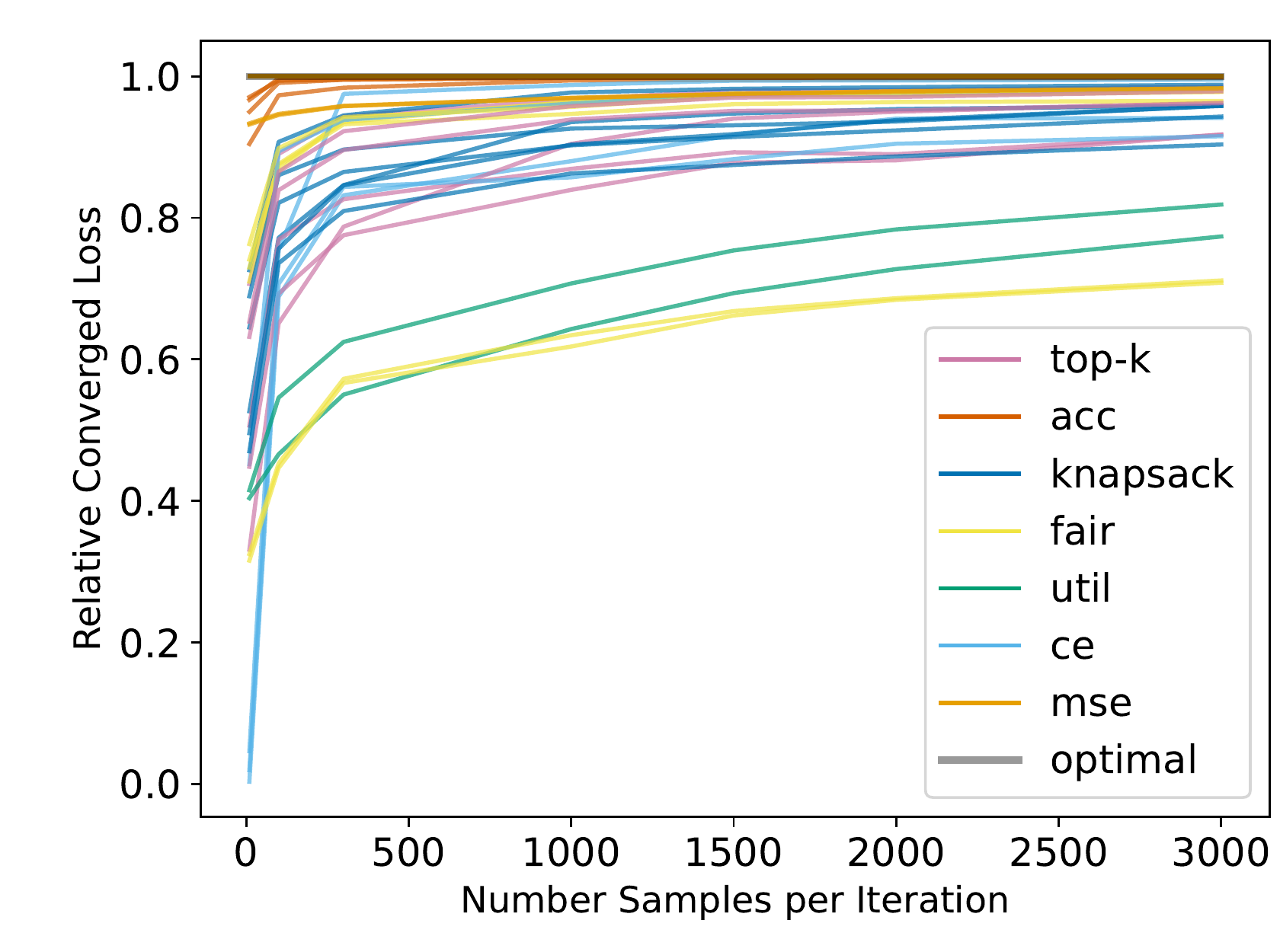
The flat line at 1.0 is the answer of Pyomo/IPOPT. Each colored curve is the method's result as a share of it.
Moving right, more problems are sampled per step. Most curves end above 0.8.
Three curves end below 0.8: two for fair and one for util. None ends below 0.6.
Pyomo/IPOPT was used as the reference. Most curves, 87%, ended above 80% of its value. §4.3 All ended above 60%. §4.3 Every curve rose as more problems were sampled per step. §4.3
The theory guarantees less. The method is sure to reach at least 1/e, about 37%, of the true worst-case loss, up to a small error. That is the largest average decision loss any shift in the set can cause. §4.3 §3 So the search did much better than its guarantee in this test. §4.3
Why can the worst case for 1-accuracy be mild for top-k?
Why does the worst case for the fairness-based loss upweight white employed people with high predictions?
A high prediction puts them in the top k, so they get help they do not need. Non-white unemployed people with high predictions are served correctly. That gap in treatment between racial groups is what the fairness-based loss measures. §4.3
chapter 5
What this does not show
The paper's version in the proceedings has no limits section. These points are drawn from its setup.
- Three tasks, one data source. All results come from US census tasks, with states as groups. §4 Other kinds of allocation were not tested.
- Shift size is a choice. The two limits on the divergence were set by the authors to give meaningful constraints. App.D Other limits may give other worst cases.
- Exactness checked only on small groups. The comparison with an exact solver used 8 people per group. The main runs used 40. App.D
- A worst case is not a forecast. The method finds the most harmful change within the set. It does not say how likely that change is. §2
The paper says its method finds worst cases for allocation much better than DRO-like methods. §4.3 Its evidence is Figure 1: each loss's own search beats the others on that loss. The paper does not report a separate head-to-head run against a published DRO method.
Why does the user's choice of shift size matter?
Does the method say how likely the worst case is?
No. It finds the most harmful change within the allowed set, not the most probable one. §2
chapter 6
Questions people ask
Short answers to common questions. Each one points back to the paper.
What is a distribution distribution shift?
A model is trained on one set of data and then used on another. The paper calls the difference a distribution shift. §1
What is a worst-case distribution shift distribution?
It is the change in the data that makes a model's loss largest, within a set size. §2 The size is set by capping a divergence, which measures how far a new weighting moves from the empirical distribution. §3
How is distributionally robust optimization different from the paper's method?
Distributionally robust optimization looks for the worst data mix. It counts loss one person at a time. §1 §2 The paper searches for the worst case of the decision loss instead. That loss scores the decision made from all the predictions together. §3 §4.3
Why does a worst case for accuracy miss harm to decisions?
Many errors do not change who gets the resource, so a model can be more robust than expected. Small errors near the cutoff can change who is treated, so it can also be less robust. §1 On one income task, the worst case for 1-accuracy reached only 0.14 of the worst top-k loss. Figure 1
What is resource allocation here?
Predictions decide who gets a scarce resource. §1 The paper's example is an emergency room with a limited treatment. In top-k, the k people with the highest predictions get the resource. §1 §4.1
keep it
This page has 10 check-yourself questions. The review page asks them again after 1, 3, 7 and 21 days, one at a time. You can also download them for Anki.
chapter 7
Words to know
Hover or tap any underlined word on the page to see its entry. These are the terms this page uses, in the order it introduces them.
- distribution shift (change in the data)
- The data a model meets after it is put to use differs from the data it was trained on."distribution shifts, which are characterized by statistical differences between the data encountered during deployment and the data used in training" (§1)
- worst-case distribution shift (most harmful change)
- Among all changes to the data up to a set size, the one that makes a chosen loss as large as it can be."we consider the challenge of identifying the worst-case distribution shift for allocation performance within a constrained set parameterized by the total size of the shift allowed" (§2)
- resource allocation (sharing out a limited resource)
- Predictions decide who among a group gets something there is not enough of, such as a treatment or a program."resource allocation settings, in which predictions are used to prioritize individuals within a given decision problem to receive a scarce resource" (§1)
- predict-then-optimize
- First a model predicts numbers, then those numbers are fed into a decision problem that picks the best action."Predict-then-optimize describes settings in which a predictive model first predicts a cost vector from a vector of features, and then, the predicted cost vector is used as a set of parameters for an optimization problem." (App. A)
- optimization instance (decision group)
- One group of people for whom one allocation decision is made together, such as the patients of one day at an emergency room, or people from one US state."Formally, decisions are made on the level of optimization instances that consist of many individuals." (§1)
- decision loss (cost of the wrong choice)
- How much worse the decision made from the predictions is than the decision that would be made with the true outcomes."We define the decision loss on a given instance to be the regret relative to if the true Y were known" (§2)
- regret
- The value of the best decision minus the value of the decision actually made."Common choices for g may include subtraction (regret) or division (relative regret)." (§2)
- top-k
- Give the resource to the k people with the highest predictions. Count how many of them truly needed it."First, we look at top-k, where the decision maker has k units of the resource available per instance and the objective function is the number of individuals with true label 1 who receive the resource." (§4.1)
- knapsack
- Like top-k, but each person has a cost and the total cost has a cap. Here the cost grows with years of education."the decision maker's objective is the same as the top-k setting but they are subject to a knapsack constraint instead of a simple budget" (§4.1)
- distributionally robust optimization (training for the worst case)
- A family of methods that train or test a model against the worst data mix within a set size. They usually measure loss one person at a time."previous works in the distributionally robust optimization (DRO) literature seek to minimize worst-case loss over a feasible set of distributions" (§1)
- empirical distribution (the data as observed)
- Each observed person or group counts with equal weight, exactly as in the data."we adapt the common strategy of using the empirical distribution over the samples" (§3)
- divergence (distance between mixes)
- A number that says how far one way of weighting the data is from another. The paper caps it to limit the size of a shift."where D is a standard divergence on distributions (e.g., the χ2 divergence) and ρind is a parameter chosen by the user to control the amount of distribution shift allowed at the individual level" (§3)
- hierarchical model (two-level model of the data)
- First pick a group (one decision group), then pick its people. A shift can change both how often each group appears and who is in it."we use a hierarchical model for the data generating distribution to capture the optimization instance-style of modeling real-world allocation tasks" (§1, §3)also called in the paper: two-level generative model
- DR-submodular (diminishing-returns shaped)
- A function where each extra bit of any input adds less than the bit before. This shape lets simple step-by-step methods reach a solution with a known quality."A twice-differentiable function f : X → Y is DR-submodular if all entries of the Hessian matrix are non-positive." (§3, Definition 3.2)
- Frank-Wolfe algorithm
- A step-by-step method: at each step, find the allowed direction that raises the objective most, and move a small way toward it."we utilize an adaptation of their non-monotone Frank-Wolfe variant in order to solve the above DR-submodular problems" (§3)
- gradmax
- The inner step of the method: find the allowed weighting that points most in the direction the loss rises."Our algorithm includes a subroutine called gradmax, which maximizes the dot product over the feasible set of viable allocations and the gradients of the objective function w.r.t. the optimization variables." (§3)
- folktables
- A public package of US Census survey tasks, such as predicting employment or income.§4
- cross entropy loss
- A standard per-person loss for yes-or-no predictions. It is large when the model is confident and wrong."We also look at the cross entropy loss (CE) over individuals." (§4.1)
- mean squared error
- The average of the squared gap between predicted and true income."For the income regression task, we look at mean squared error (MSE)" (§4.1)
- Smart Predict-then-Optimize loss
- A training loss from earlier work that trains a model for the decision it feeds, here the knapsack decision."Smart Predict-then-Optimize loss (SPO) with knapsack as the underlying decision task" (§4.2)
- decision-blind metric (one-person-at-a-time score)
- A loss that adds up errors person by person and ignores the decision made from the predictions."We refer to decision-blind metrics that do not consider the relative predictive model outputs; these metrics can be expressed as a sum of losses over individuals." (§4.3)
- 1-accuracy (error rate)
- The share of people the model labels wrong. The figures call it acc."For the binary prediction tasks, we look at 1-accuracy, or the misclassification rate over individuals." (§4.1)
- decision-based metric (decision score)
- A loss that looks at the decision made from all the predictions together, such as who gets the resource."We refer to decision-based metrics as metrics that consider the relative predictive model outputs and/or individual-level features in an optimization problem." (§4.3)
- fairness-based loss (unfairness score)
- Take the top-k decision, see what share of people who needed it got it in each racial group, and measure how unequal those shares are."We calculate the true positive rate (TPR) over all distinct racial subgroups in the optimization instance, and calculate a Gini coefficient using these TPRs as a measure of unfairness of treatment over racial groups." (§4.1)
- utility-based loss (welfare score)
- A budget of money goes to people with low predicted income. The loss is how much less welfare this gives than the best split."a utility-based loss, where a decision maker seeks to maximize the Nash social welfare function of income, divided by a constant, over individuals" (§4.1)
- Pyomo/IPOPT
- Pyomo is a modeling tool and IPOPT a standard solver for smooth optimization problems. The paper uses them as a reference answer on small problems.§4.3